---
title: "Linear Regression Model"
description: ""
number-sections: true
title-block-banner: "#00868B"
title-block-banner-color: "white"
crossref:
fig-title: "Figure"
tbl-title: "Table"
---
```{r}
#| include: false
library(tidyverse)
student_performance <- read_csv("datasets/StudentPerformanceFactors.csv")
student_performance <- student_performance |>
mutate(
Extracurricular_Activities = case_when(
Extracurricular_Activities == "Yes" ~ TRUE,
Extracurricular_Activities == "No" ~ FALSE,
TRUE ~ NA
),
Internet_Access = case_when(
Internet_Access == "Yes" ~ TRUE,
Internet_Access == "No" ~ FALSE,
TRUE ~ NA
),
Learning_Disabilities = case_when(
Learning_Disabilities == "Yes" ~ TRUE,
Learning_Disabilities == "No" ~ FALSE,
TRUE ~ NA
)
) |>
rename(
hours_studied = Hours_Studied,
attendance = Attendance,
parental_involvement = Parental_Involvement,
access_to_resources = Access_to_Resources,
extracurricular_activities = Extracurricular_Activities,
sleep_hours = Sleep_Hours,
previous_scores = Previous_Scores,
motivation_level = Motivation_Level,
internet_access = Internet_Access,
tutoring_sessions = Tutoring_Sessions,
family_income = Family_Income,
teacher_quality = Teacher_Quality,
school_type = School_Type,
peer_influence = Peer_Influence,
physical_activity = Physical_Activity,
learning_disabilities = Learning_Disabilities,
parental_education_level = Parental_Education_Level,
distance_from_home = Distance_from_Home,
gender = Gender,
exam_score = Exam_Score,
)
```
::: {.callout-note icon="false" collapse="true" title="Dataset: `student_performance`"}
The `student_performance` dataset is a large educational dataset that seeks to capture the many different factors that can influence how well a student performs on their final exam. The fundamental research question behind this dataset is: *what predicts student academic achievement, and how strongly does each factor contribute?* This dataset is publicly available on the Kaggle platform, where it was published under the title [Student Performance Factors](https://www.kaggle.com/datasets/lainguyn123/student-performance-factors). The dataset contains 6607 observations, where each observation represents one individual student. For each student, 20 variables have been recorded. One of these variables is the outcome we want to predict (dependent variable), and the remaining 19 are potential predictors (independent variables). The variables are as follows:
- `hours_studied` records how many hours per week each student dedicates to studying,
- `attendance` represents the percentage of classes each student attended during the course,
- `parental_involvement` describes the degree to which a student's parents are involved in their education within the three levels (Low, Medium, and High),
- `access_to_resources` indicates the level of access a student has to educational resources such as textbooks, computers, or online materials within the three levels (Low, Medium, and High),
- `extracurricular_activities` records whether the student participates in extracurricular activities (`TRUE` or `FALSE`),
- `sleep_hours` records the average number of hours of sleep the student gets per night,
- `previous_scores` captures the student's scores from prior academic assessments,
- `motivation_level` captures the student's self-reported level of motivation within the three categories (Low, Medium, and High),
- `internet_access` indicates whether the student has access to the internet (`TRUE` or `FALSE`),
- `tutoring_sessions` records the number of tutoring sessions the student attended,
- `family_income` records the economic status of the student's family, categorized as Low, Medium, or High,
- `teacher_quality` describes the perceived quality of the student's teachers, categorized as Low, Medium, or High,
- `school_type` indicates whether the student attends a public or private school,
- `peer_influence` describes the nature of the influence the student's peer group has on their academic behavior, and it has three levels (Negative, Neutral, and Positive),
- `physical_activity` measures how many hours per week the student spends on physical activities,
- `learning_disabilities` records whether the student has been diagnosed with any learning disabilities (`TRUE` or `FALSE`),
- `parental_education_level` captures the highest level of education achieved by the student's parents, with categories including High School, College, and Postgraduate.
- `distance_from_home` indicates how far the student lives from their school, categorized as Near, Moderate, or Far,
- `gender` records the student's gender as either Male or Female,
- `exam_score` records the score that each student achieved on their final exam.
```{r}
# Pregled podataka
glimpse(student_performance)
```
:::
**Linear regression** is one of the oldest, most fundamental, and most widely used methods in statistics and statistical learning. Despite its simplicity, it remains an essential tool for anyone working with data, especially in the social sciences. The core idea behind linear regression is straightforward: we want to understand and quantify the relationship between one or more explanatory variables and a single outcome variable. More specifically, linear regression assumes that the relationship between the dependent and the independent variable can be described, at least approximately, by a straight line - or in the case of multiple predictors, by a flat surface (a hyperplane) in higher-dimensional space.
The purpose of linear regression is twofold. First, it serves an explanatory purpose: it helps us understand which factors are associated with the outcome and how strongly each factor contributes, while holding the other factors constant. Second, it serves a predictive purpose: once we have estimated the relationship, we can use it to predict the outcome for new observations based on their predictor values.
The simplest form of linear regression involves just one independent variable. This is called **simple linear regression**. Mathematically, it takes the form:
$$
Y \approx \beta_0 + \beta_1X
$$
In this equation, $Y$ is the **dependent variable** - the outcome we want to predict. In our example, $Y$ is, for example, the variable `exam_score`. $X$ is the **independent variable** - the factor we believe is related to the outcome. For instance, $X$ could be `hours_studied`. The symbol $\beta_0$ is called the **intercept**. It represents the expected value of $Y$ when $X$ equals zero. In our context, it would represent the expected exam score for a hypothetical student who studies zero hours. The symbol $\beta_1$ is called the **slope**. It represents the average change in $Y$ that is associated with a one-unit increase in $X$. In our example, it tells us how many additional points on the exam a student can expect to gain for each additional hour of studying. Together, intercept and slope are called the **model coefficients or parameters**.
Of course, in real life we do not know the true values of $\beta_0$ and $\beta_1$. We must estimate them from the data. Once we have estimated these coefficients - and we denote the estimates with a hat symbol as $\hat{\beta}_0$ and $\hat{\beta}_1$ - we can write our prediction equation as: $y = \hat{\beta_0} + \hat{\beta_1}x$. Here, $\hat{y}$ is the predicted value of the response for a given value $x$ of the predictor. The hat symbol indicates that we are dealing with an estimate rather than a true and known quantity.
In practice, a single predictor is rarely sufficient to explain all the variation in the response. A student's exam score is not determined by study hours alone - attendance, prior academic performance, tutoring, and many other factors play a role. **Multiple linear regression** extends the simple model to accommodate several predictors simultaneously. The general formula is:
$$
Y = \beta_0 + \beta_1X_1 + \beta_2X_2 + ... + \beta_pX_p + \epsilon
$$
In this equation, $X_1$, $X_2$, $X_3$, ..., $X_p$ represent different independent variables, and $\beta_1$, $\beta_2$, ..., $\beta_p$ are their corresponding slope coefficients. Each coefficient represents the average change in $Y$ associated with a one-unit increase in the predictor, while **holding all other predictors constant** which distinguishes multiple regression from simply running many separate simple regressions. The term $\epsilon$ represents the **error term** - it captures everything that our model does not explain, including the influence of unmeasured variables, measurement error, and the inherent randomness in human behavior.
This model allows us to estimate the unique contribution of each predictor to the exam score. For instance, $\beta_1$ tells us the expected change in exam score for each additional hour of study, after accounting for the effects of attendance, previous scores, sleep, tutoring, and physical activity. This is fundamentally different from simple linear regression, where $\beta_1$ would capture the total association between study hours and exam scores without adjusting for any other factor.
## Estimating the Coefficients of Parameters
The key question is how do we actually find the best values for our coefficients of parameters estimates. The answer lies in the **least squares method**, which is the most common approach for fitting a linear regression model. The basic idea is intuitive: we want our predicted values to be as close as possible to the actual observed values for every observation in our dataset.
For each observation, the difference between the observed value and the predicted value is called the **residual**, denoted $e_i = y_i - \hat{y}_i$. The residual tells us how much our model's prediction misses the actual outcome for that particular student. Some residuals will be positive (when the model underpredicts) and some will be negative (when the model overpredicts).
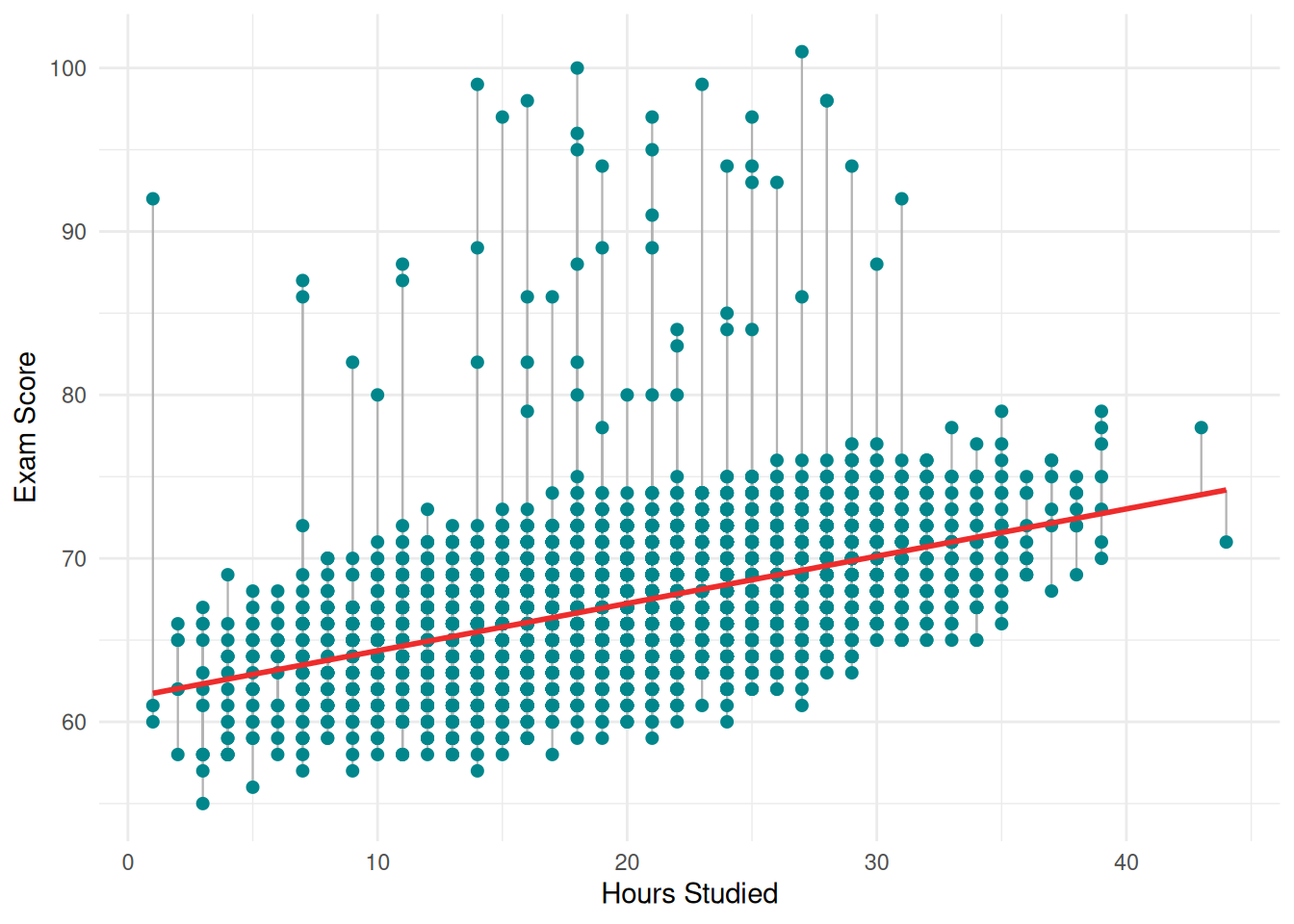
```{r}
#| fig.cap: "Simple Linear Regression: Exam Score ~ Hours Studied"
#| echo: false
#| warning: false
#| message: false
simple_model <- lm(exam_score ~ hours_studied, data = student_performance)
student_performance$predicted <- predict(simple_model)
ggplot(student_performance, aes(x = hours_studied, y = exam_score)) +
geom_segment(aes(xend = hours_studied, yend = predicted), color = "grey70", linewidth = 0.4) +
geom_point(color = "#00868B", size = 1.8) +
geom_smooth(method = "lm", se = FALSE, color = "#EE2C2C", linewidth = 1) +
labs(x = "Hours Studied", y = "Exam Score") +
theme_minimal()
```
To get an overall measure of how well the model fits all the data, we cannot simply add up the residuals, because the positive and negative ones would cancel each other out. Instead, we square each residual and then sum them all up. This quantity is called the **residual sum of squares** (RSS):
$$
RSS = e_1^2 + e_2^2 + ... + e_n^2 = \sum(y_i - \hat{y}_i)^2
$$
The least squares method chooses the coefficient estimates that minimize this RSS. In other words, the least squares approach finds the line (in simple regression) or the hyperplane (in multiple regression) that makes the total squared prediction error as small as possible. This is a well-defined mathematical optimization problem, and the solution can be computed using calculus. For simple linear regression, the formulas for the minimizers have a closed-form expression:
$$
\begin{array}{cc}
\hat{\beta}_0 = \bar{y} - \hat{\beta}_1 \bar{x}
&
\hat{\beta}_1 = \frac{\sum_{i = 1}^n (x_i - \bar{x})(y_i - \bar{y})} {\sum_{i = 1}^n (x_i - \bar{x})^2}
\end{array}
$$
By this, the least squares method provides a principled, objective way to estimate the model parameters. It does not require any subjective judgment about what the "best" line should look like, but simply finds the line that minimizes the total squared distance between the observed data points and the fitted line.
To fit a simple linear regression model in R, we use the `lm()` function. The syntax follows the pattern `lm(response ~ predictor, data = dataset)`. The tilde symbol (`~`) can be read as "*is modeled as a function of*". The `lm()` fits the model by computing the least squares coefficient estimates, and the output shows the estimated parameters of a simple linear regression model.
The `summary()` function then provides a detailed output that includes the estimated coefficients, their standard errors, t-statistics, p-values, the residual standard error, and the $R^2$ statistic. The `confint()` function computes the 95% confidence intervals for each coefficient estimate, which tell us the range of plausible values for the true population parameters.
::: {.callout-tip icon="false" collapse="true" title="Example: Simple Linear Regression"}
```{r}
simple_model <- lm(
    exam_score ~ hours_studied,
    data = student_performance
)

summary(simple_model)$coefficients[, "Estimate"]
```
For simple linear regression of `exam_score` onto `hours_studied`, the intercept is estimated at 61.4570. This means that when `hours_studied` equals zero, the model predicts an exam score of approximately 61.46 points. In substantive terms, a hypothetical student who does not study at all would be expected to score about 61.5 on the exam, according to this model. This makes intuitive sense - students would still have some baseline level of knowledge from attending classes, even without additional study outside the classroom. The slope for `hours_studied` is estimated at 0.289. This tells us that for each additional hour of study per week, a student's exam score is expected to increase by approximately 0.29 points, on average. So a student who studies 10 hours more per week than another student would be expected to score about 2.89 points higher on the exam.
:::
For the multiple linear regression model, we simply add more predictors to the right side of the formula, separated by the `+` sign: `response ~ predictor 1 + predictor 2 + predictor 3 + ...`. This tells R to fit a model that predicts dependent variable using all quantitative predictors simultaneously. The least squares method will estimate a separate slope coefficient for each predictor, along with a single intercept, by minimizing the total RSS across all observations.
::: {.callout-tip icon="false" collapse="true" title="Example: Multiple Linear Regression"}
```{r}
multiple_model <- lm(
    exam_score ~ hours_studied + attendance + previous_scores + sleep_hours + tutoring_sessions + physical_activity,
    data = student_performance
)

summary(multiple_model)$coefficients[, "Estimate"]
```
The intercept is now estimated at 40.927. This is substantially lower than in the simple model (61.46), which makes sense. In the simple model, the intercept represented the predicted score when only `hours_studied` was zero. In the multiple model, the intercept represents the predicted score when all six predictors are on their average value. Such a student is of course entirely hypothetical and unrealistic, which is why we should not over-interpret the intercept in multiple regression.
The coefficient for `hours_studied` is 0.292, which is remarkably similar to its value in the simple regression (0.289). This tells us something important: the relationship between study hours and exam scores is robust - it persists even after we account for the effects of attendance, prior scores, sleep, tutoring, and physical activity. In substantive terms, holding all other factors constant, each additional hour of study per week is associated with an increase of about 0.29 points on the exam.
The coefficient for `attendance` is 0.198, meaning that each additional percentage point of class attendance is associated with about 0.20 additional points on the exam, after controlling for the other variables. To put this in perspective, a student who attends 90% of classes versus one who attends 70% of classes would be expected to score about 3.96 points higher, all else being equal. The coefficient for `previous_scores` is 0.048. This means that for each additional point a student earned on their previous assessments, their exam score is expected to increase by about 0.048 points, holding other factors constant. A student whose prior scores are 20 points higher than another student's would be expected to score only about 0.96 points higher on this exam. This suggests that while past performance does predict future performance, its incremental contribution is small once study habits and attendance are already accounted for. The coefficient for `sleep_hours` is -0.018. The negative sign suggests that more sleep is associated with slightly lower exam scores, meaning that each additional hour of sleep per night is associated with a decrease of about 0.02 points on the exam, after controlling for the other variables. The coefficient for `tutoring_sessions` is 0.494, the largest individual slope coefficient in the model. Each additional tutoring session is associated with about half a point increase on the exam. The coefficient for `physical_activity` is 0.144, meaning that each additional hour per week of physical activity is associated with about 0.14 additional exam points, after controlling for the other variables.
:::
## Accuracy of the Coefficient Estimates
An important issue that arises here concerns the **accuracy of detected estimates**. If a different sample of students were collected, the coefficient estimates might not remain identical but could vary due to sampling variability. This raises the broader problem of statistical uncertainty: the observed relationship between `study_hours` and `exam_scores` may reflect a genuine positive association in the population, yet it is also possible that the estimated effect is partly driven by random variation specific to the analysed sample. Consequently, the reliability and inferential validity of the estimated coefficients depend on the extent to which sampling error can be ruled out as a substantive explanation of the observed effect.
When we write the linear regression model as $Y = \beta_0 + \beta_1X + \epsilon$, we are making a statement about the true, underlying relationship between $X$ and $Y$ in the entire population - not just in our particular sample. The coefficients $\beta_0$ and $\beta_1$ are the true population parameters, which we will never know exactly. The term $\epsilon$ is the **error term**, and it represents everything that our model fails to capture. There are several reasons why the error term exists. First, the true relationship between the predictor and the response may not be perfectly linear - there may be curvature or other patterns that a straight line cannot capture. Second, there may be other variables that influence the response but are not included in our model. Third, there is always some inherent randomness and measurement error in any data we collect. The error term absorbs all of these sources of discrepancy between what our model predicts and what actually happens.
In our `student_performance` example, even if we knew the exact true values of $\beta_0$ and $\beta_1$ for the relationship between `hours_studied` and `exam_score` in the entire population of all students, we still could not predict any individual student's exam score perfectly. Some students who study 20 hours per week will score higher than the regression line predicts, and others will score lower. These deviations are captured by $\epsilon$. We typically assume that the error term has a mean of zero (meaning the model does not systematically overpredict or underpredict), that the errors for different observations are independent of each other, and that the errors have a constant variance $\sigma^2$ across all values of $X$.
The true population regression line, $Y = \beta_0 + \beta_1X$, represents the best linear summary of the relationship between $X$ and $Y$ in the entire population. Our estimated regression line, $\hat{y} = \hat{\beta}_0 + \hat{\beta}_1x$, is our best approximation of this population line based on the data we have. The key insight is that $\hat{\beta}_0$ and $\hat{\beta}_1$ are estimates of the true parameters, computed from one particular sample. If we were to draw a different random sample of 6,607 students, we would get slightly different estimates. This variability across samples is what motivates the need for standard errors, confidence intervals, and hypothesis tests - they allow us to quantify how much uncertainty surrounds our estimates.
### Standard Errors
The **standard error of a coefficient estimate** measures how much that estimate would vary if we repeatedly drew new samples from the same population and re-estimated the model each time. In other words, it quantifies the precision of our estimate. A small standard error means that our estimate is very precise - different samples would give us very similar coefficient values. A large standard error means that our estimate is imprecise - it might change substantially from sample to sample.
The standard error of the coefficients or parameters in linear regression is given by the formulas:
$$
\begin{array}{cc}
SE(\hat{\beta}_0) = \sigma^2 [\frac{1}{n} + \frac{\bar{x}^2}{\sum_{i =1}^n(x_i - \bar{x})^2}]
&
SE(\hat{\beta}_1) = \frac{\sigma}{\sum_{i=1}^n(x_i - \bar{x})^2}
\end{array}
$$
This formulas reveals two important things. First, the standard error depends on $\sigma$, the standard deviation of the error term. If there is a lot of noise in the data (large $\sigma$), then the estimated slope will be less precise, because the true signal is harder to detect amid the noise. Second, the standard error depends on the spread of the predictor values. When the $x_i$ values are more spread out (that is, when the total squared deviation of the $x$ values from their mean is large), the standard error is smaller. Intuitively, this makes sense: if we observe students who study anywhere from 1 to 44 hours per week, we have a much better basis for estimating the slope than if all students studied between 19 and 21 hours. A wider range of predictor values gives us more "leverage" to pin down the relationship. In practice, the true value of $\sigma$ is unknown and must be estimated from the data. This estimate is the residual standard error (RSE).
::: {.callout-tip icon="false" collapse="true" title="Example: Standard Errors"}
```{r}
summary(simple_model)$coefficients[, "Std. Error"]
```
Looking at our simple regression, the standard error for the `hours_studied` coefficient is 0.00715. This is very small relative to the coefficient estimate of 0.289, which tells us that our estimate is highly precise. The reason for this high precision is our large sample size combined with a good spread in study hours.
```{r}
summary(multiple_model)$coefficients[, "Std. Error"]
```
In the multiple regression model, the standard error for `hours_studied` is even smaller at 0.00507. This decrease occurs because the multiple model has a lower RSE, which means there is less unexplained noise once we account for the additional predictors - and less noise translates directly into more precise coefficient estimates. The standard errors for the other coefficients in the multiple model tell a similar story. `attendance` has a standard error of 0.00263, `previous_scores` has 0.00211, `sleep_hours` has 0.0207, `tutoring_sessions` has 0.0247, and `physical_activity` has 0.0294. Notice that `sleep_hours` has a relatively large standard error compared to its coefficient estimate (-0.018), which foreshadows the fact that this coefficient will not be statistically significant - the estimate is so imprecise relative to its magnitude that we cannot confidently distinguish it from zero.
:::
A **confidence interval** provides a range of plausible values for the true population parameter. The 95% confidence interval for a regression coefficient is constructed using the formula:
$$
\hat{\beta}_j \pm 2 \times SE(\hat{\beta}_j)
$$
More precisely, the multiplier is not exactly 2 but rather the 97.5th percentile of the t-distribution with $n-p-1$ degrees of freedom, where $n$ is the sample size and $p$ is the number of predictors. The interpretation of a 95% confidence interval is as follows: if we were to repeat the study many times, drawing a new random sample each time and computing a 95% confidence interval from each sample, then 95% of those intervals would contain the true population parameter. It is important to note that this does not mean there is a 95% probability that the true parameter lies within our specific interval - the true parameter is a fixed value, not a random quantity. Rather, the 95% refers to the long-run reliability of the procedure.
::: {.callout-tip icon="false" collapse="true" title="Example: Confidence Intervals"}
```{r}
confint(simple_model)
```
In the simple regression, the 95% confidence interval for the `hours_studied` coefficient is [0.275, 0.303]. This interval is narrow, reflecting the high precision of our estimate, and it lies entirely above zero. We can therefore state with 95% confidence that the true effect of one additional hour of study falls somewhere between 0.275 and 0.303 points on the exam.
```{r}
confint(multiple_model)
```
In the multiple regression, the confidence intervals are similarly informative. For `attendance`, the interval is [0.193, 0.203], meaning we are 95% confident that each additional percentage point of attendance is associated with between 0.19 and 0.20 additional exam points, after controlling for the other predictors. For `tutoring_sessions`, the interval is [0.445, 0.542], and for `physical_activity` it is [0.086, 0.202] - all comfortably above zero. The critical case is `sleep_hours`, whose confidence interval is [-0.059, 0.023]. Because this interval spans from a negative value to a positive value, crossing zero in the middle, we cannot determine whether the true effect of sleep hours on exam scores is positive, negative, or simply zero.
:::
### Hypothesis Testing and the t-Statistic
**Hypothesis testing** provides a formal framework for determining whether the relationship we observe in our sample is likely to reflect a real relationship in the population, or whether it could plausibly be due to random chance. In linear regression, the most common hypothesis test for each coefficient is:
- **The null hypothesis** ($H_0$): $\beta_j = 0$, meaning there is no relationship between $X$ and $Y$.
- **The alternative hypothesis** ($H_a$): $\beta_j \neq 0$, meaning there is some relationship between $X$ and $Y$.
If the null hypothesis is true and the predictor truly has no effect on the response, then the true slope is zero, and any non-zero slope we estimate from our sample is simply due to random noise. The **t-statistic** allows us to assess how likely this scenario is, and it can be computed as:
$$
t = \frac{\hat{\beta}_j}{SE(\hat{\beta}_j)}
$$
This is simply the coefficient estimate divided by its standard error. It measures how many standard errors the coefficient estimate is away from zero. A t-statistic close to zero means that the coefficient estimate is small relative to its uncertainty, which is consistent with the null hypothesis. A t-statistic far from zero (either very positive or very negative) means that the coefficient estimate is large relative to its uncertainty, which provides evidence against the null hypothesis.
Under the null hypothesis, the t-statistic follows a t-distribution with $n-p-1$ degrees of freedom. For large samples, the t-distribution is virtually identical to the normal distribution, so a t-statistic beyond roughly $\pm2$ is generally considered statistically significant at the 5% level, and beyond roughly $\pm2,75$ at the 1% level.
::: {.callout-tip icon="false" collapse="true" title="Example: t-statistics"}
```{r}
summary(simple_model)$coefficients[, "t value"]
```
In the simple regression model, the t-statistic for `hours_studied` is 40.44. This means the coefficient estimate is more than 40 standard errors away from zero. To put this in perspective, if study hours truly had no effect on exam scores, observing a t-statistic this large would be essentially impossible - it would be like flipping a fair coin and getting heads 40 times in a row, except far less likely even than that. This gives us overwhelming evidence that the relationship between study hours and exam scores is real.
```{r}
summary(multiple_model)$coefficients[, "t value"]
```
In the multiple regression model, the t-statistics reveal a clear hierarchy of evidence. `attendance` has the largest t-statistic at 75.26, making it the most precisely estimated and most strongly significant predictor. `hours_studied` follows with 57.52, then `previous_scores` at 22.81, `tutoring_sessions` at 20.00, and `physical_activity` at 4.89. All of these are far beyond any conventional significance threshold. The exception, as we have seen, is `sleep_hours`, with a t-statistic of only -0.871. This value is well within the range we would expect to see even if the true coefficient were zero - it is less than one standard error away from zero, which is entirely unremarkable.
:::
### The p-Value
The **p-value** is the probability of observing a t-statistic as extreme as the one we actually computed, assuming that the null hypothesis is true. In other words, it answers the question: *if there were truly no relationship between this predictor and the response, how surprising would our observed result be?*
A small p-value (typically below 0.05) indicates that the observed result would be very surprising under the null hypothesis, and we therefore reject the null hypothesis in favor of the alternative. A large p-value indicates that the observed result is not particularly surprising under the null hypothesis, and we therefore fail to reject it. It is important to emphasize that "failing to reject" is not the same as "accepting" the null hypothesis - it simply means we do not have enough evidence to conclude that a relationship exists.
::: {.callout-tip icon="false" collapse="true" title="Example: p-values"}
```{r}
summary(simple_model)$coefficients[, "Pr(>|t|)"]
```
In our simple regression output, the p-value for `hours_studied` is 1.286349e-319, and it is so close to zero that for all practical purposes it means the probability of observing our results by chance alone is essentially zero. Therefore, we have overwhelming evidence to reject the null hypothesis and conclude that there is a statistically significant relationship between hours studied and exam scores.
```{r}
summary(multiple_model)$coefficients[, "Pr(>|t|)"]
```
In the multiple regression, the p-values for `hours_studied`, `attendance`, `previous_scores`, and `tutoring_sessions` are all 0.000000e+00, and the p-value for `physical_activity` is 1.033431e-06. All of these are far below any conventional significance threshold, providing overwhelming evidence that these predictors are genuinely related to exam scores.
The p-value for `sleep_hours`, however, is 3.836647e-01. This means that if sleep hours truly had no effect on exam scores, there would be about a 38.4% probability of observing a coefficient estimate as far from zero as the one we found. In other words, our observed result is entirely unsurprising under the null hypothesis - it is the kind of result we would expect to see by random chance alone roughly 38 times out of 100. We therefore have no grounds to reject the null hypothesis for `sleep_hours`, and we conclude that this variable does not have a statistically significant linear relationship with exam scores in this model.
:::
## Model Fit
In the previous section, we focused on assessing the accuracy of individual coefficient estimates - asking whether each specific predictor is significantly related to the response. Now we shift our perspective and ask how well the model as a whole fits the data. In other words, we have to examine how good it is at capturing the actual patterns in student exam scores.
To answer these questions, we rely on three complementary statistics that appear at the bottom of every regression summary in R: the residual standard error (RSE), the $R^2$ statistic, and the F-statistic. Each of these measures provides a different lens through which to evaluate the overall quality of the model, and together they give us a well-rounded picture of model performance.
### Residual Standard Error
The **Residual Standard Error** (RSE) is perhaps the most intuitive measure of model accuracy, because it is expressed in the same units as the dependent variable. It estimates the standard deviation of the error term - that is, it tells us the typical size of the prediction errors our model makes. The RSE is computed using the formula:
$$
RSE = \sqrt{\frac{RSS}{n - p - 1}}
$$
In this formula, RSS is the residual sum of squares, $n$ is the number of observations, and $p$ is the number of predictors. The denominator uses $n - p - 1$ rather than simply $n$ because we have used up $p + 1$ degrees of freedom in estimating the intercept and the $p$ slope coefficients. This correction ensures that the RSE is an unbiased estimate of the true error standard deviation $\sigma$. The concept of degrees of freedom can be understood intuitively: each parameter we estimate "uses up" one piece of information from the data, leaving fewer independent pieces of information available to estimate the error variance.
::: {.callout-tip icon="false" collapse="true" title="Example: Residual Standard Error"}
```{r}
summary(simple_model)$sigma
```
In our simple regression model, the RSE is 3.483. This means that, on average, the actual exam scores deviate from the scores predicted by the model by approximately 3.48 points. Given that the mean exam score in our dataset is 67.24, we can express this as a percentage error of about 5.18% (3.483 / 67.24 × 100). Whether this level of error is acceptable depends entirely on the context of the research. From a pure prediction standpoint, it also tells us that our simple model leaves a lot of room for improvement - knowing only how many hours a student studies does not allow us to predict their exam score with great precision.
```{r}
summary(multiple_model)$sigma
```
In our multiple regression model, the RSE drops to 2.467. This represents a substantial improvement over the simple model - the average prediction error has decreased by about 29%, from 3.48 to 2.47 points. The percentage error relative to the mean is now approximately 3.67% (2.467 / 67.24 × 100). This decrease makes intuitive sense: by adding attendance, previous scores, tutoring sessions, and physical activity to the model, we have incorporated additional information that helps explain why some students score higher than others. The model now captures more of the systematic patterns in the data, leaving less to the error term.
:::
One important limitation of the RSE is that it is measured in the units of the response variable, which makes it difficult to compare across different studies or datasets with different response scales. If another researcher studied a test scored on a scale of 0 to 500, their RSE would naturally be much larger in absolute terms, even if their model were proportionally just as accurate as ours. This limitation motivates the need for a scale-independent measure of model fit, which is exactly what the $R^2$ statistic provides.
### $R^2$
The **$R^2$** statistic, also known as the coefficient of determination, is one of the most commonly reported measures of model fit in applied research. Unlike the RSE, $R^2$ is a proportion that always takes a value between 0 and 1, making it easy to interpret and compare across studies regardless of the scale of the response variable. $R^2$ answers a question on what fraction of the total variation in the response variable is explained by the model. To understand $R^2$, we need to consider two quantities.
The first is the **Total Sum of Squares** (TSS), defined as:
$$
TSS = \sum(y_i - \hat{y})^2
$$
This measures the total variability in the response variable before any regression is performed. It is simply the sum of the squared deviations of each observed exam score from the overall mean exam score. In our dataset, this captures the full extent to which students' exam scores differ from one another. Some of this variation is systematic and some of it is random noise.
The second quantity is the **Residual Sum of Squares** (RSS), which we have already encountered:
$$
RSS = \sum(y_i - \hat{y}_i)^2
$$
This measures the variability that remains unexplained after fitting the regression model. It is the sum of the squared residuals - the squared differences between the actual exam scores and the scores predicted by the model.
The $R^2$ statistic is then defined as:
$$
R^2 = \frac{(TSS - RSS)}{TSS} = 1 - \frac{RSS}{TSS}
$$
The numerator, TSS - RSS, represents the amount of variability in the response that is explained by the regression - it is the reduction in prediction error achieved by using the model instead of simply predicting the mean for every student. Dividing by TSS converts this into a proportion.
When $R^2$ is close to 1, it means that the model explains nearly all of the variation in the response. In such a case, the predicted values $\hat{y}_i$ are very close to the actual values $y_i$, and the model provides an excellent fit. When $R^2$ is close to 0, the model explains very little of the variation, and using the model is hardly better than simply predicting the mean exam score for every student. What constitutes a "good" $R^2$ depends heavily on the field of study. In the social sciences, where human behavior is inherently noisy and influenced by a vast number of interacting factors, $R^2$ values between 0.30 and 0.60 are often considered quite good for observational studies.
::: {.callout-tip icon="false" collapse="true" title="Example: R-squared"}
```{r}
summary(simple_model)$r.squared
```
In our simple regression model, $R^2$ is 0.1984. This tells us that `hours_studied` alone explains approximately 19.84% of the total variation in exam scores. In other words, about one-fifth of the differences in exam scores among students can be attributed to differences in how many hours they study. This is a meaningful finding - it confirms that study time matters - but it also reveals that roughly 80% of the variation is driven by other factors not captured in this simple model.
```{r}
summary(multiple_model)$r.squared
```
In our multiple regression model, $R^2$ jumps to 0.5982. Now the model explains approximately 59.82% of the variation in exam scores. This is a dramatic improvement - by adding attendance, previous scores, tutoring sessions, and physical activity as predictors alongside study hours, we have nearly tripled the proportion of explained variance. The remaining approximately 40% of the variation is still unexplained, presumably due to factors that are not included as quantitative predictors in this model - things like motivation level, family income, teacher quality, peer influence, and other qualitative variables in our dataset that we have not yet incorporated, as well as entirely unmeasured factors like test anxiety, the specific content of the exam, or simple luck.
:::
It is critical to understand one important caveat about $R^2$: it will always increase (or at least never decrease) when more predictors are added to the model, even if those predictors are completely unrelated to the response. This happens because adding any variable, even a random one, gives the model more flexibility to fit the training data, and the RSS can only go down or stay the same - it can never go up. This means that a high $R^2$ does not necessarily indicate a good model; it could simply reflect the fact that many predictors have been thrown in. To guard against this problem, the **adjusted $R^2$** was developed. The Adjusted $R^2$ modifies the standard $R^2$ by imposing a penalty for each additional predictor. If adding a new predictor does not reduce the RSS enough to offset the penalty for the lost degree of freedom, the adjusted $R^2$ will actually decrease, signaling that the added predictor is not contributing meaningfully.
::: {.callout-tip icon="false" collapse="true" title="Example: Adjusted R-squared"}
```{r}
summary(simple_model)$adj.r.squared
summary(multiple_model)$adj.r.squared
```
In our simple model, the adjusted $R^2$ is 0.1983, virtually identical to $R^2$ because there is only one predictor and the penalty is negligible. In our multiple model, the adjusted $R^2$ is 0.5979, also nearly identical to the regular $R^2$ of 0.5982. The fact that the adjusted $R^2$ barely differs from $R^2$ in the multiple model tells us that all six predictors (or at least most of them) are genuinely contributing to the model's explanatory power - the improvement in fit is not merely an artifact of adding more variables.
:::
It is also worth noting the connection between $R^2$ and **correlation**. In simple linear regression, $R^2$ is exactly equal to the square of the Pearson correlation coefficient r between $X$ and $Y$. In our case, $R^2$ = 0.1984 for the simple model, so the correlation between `hours_studied` and `exam_score` is $r = \sqrt{0.1984} \approx 0.445$. In multiple regression, this simple relationship no longer holds (because there are multiple predictors), but $R^2$ can be shown to equal the squared correlation between the observed values $y_i$ and the fitted values $\hat{y}_i$. This provides a nice intuitive interpretation: $R^2$ tells us how closely the model's predictions track the actual outcomes.
### F-statistic
While the t-statistic and its associated p-value allow us to test whether each individual predictor is significantly related to the response, the **f-statistic** addresses if the model as a whole is useful. Specifically, the F-statistic tests the null hypothesis that all slope coefficients in the model are simultaneously equal to zero ($H_0 \beta_1 = \beta_2 = ... = \beta_p = 0$) against the alternative hypothesis ($H_a$: at least one $\beta_j$ is non-zero).
If the null hypothesis is true, then none of the predictors have any relationship with the response, and the model is no better than simply predicting the mean for every observation. The f-statistic is computed as:
$$
F = \frac{\frac{TSS - RSS}{p}}{\frac{RSS}{n - p -1}}
$$
The numerator measures how much of the total variance the model explains, divided by the number of predictors $p$. The denominator measures how much variance remains unexplained, divided by the residual degrees of freedom. If the model is no better than chance, the numerator and denominator should be roughly equal, producing an f-statistic close to 1. If the model captures real patterns in the data, the numerator will be much larger than the denominator, producing a large f-statistic.
One might reasonably ask: why do we need the F-statistic at all when we already have individual t-tests for each coefficient? The answer lies in the multiple testing problem. When we have many predictors, each with its own t-test, the probability of finding at least one "significant" result by pure chance increases dramatically. For example, if we tested 100 completely useless predictors at the 5% significance level, we would expect about 5 of them to appear significant purely by chance. The F-statistic avoids this problem because it is a single, omnibus test that accounts for the total number of predictors. It maintains the correct overall error rate regardless of how many predictors are in the model. So the proper approach is to first check the F-statistic to determine whether the model as a whole is significant, and only then examine the individual t-statistics to identify which specific predictors are contributing.
::: {.callout-tip icon="false" collapse="true" title="Example: F-statistic"}
```{r}
summary(simple_model)$fstatistic
```
In our simple regression model, the f-statistic is 1,635 with 1 and 6,605 degrees of freedom, and the associated p-value is less than $2.2 \times 10^{16}$. Since we have only one predictor in the simple model, the f-test is equivalent to the t-test for that predictor. In fact, the f-statistic in simple regression is exactly the square of the t-statistic: $40.44^2 \approx 1,635$. The overwhelming magnitude of this f-statistic and its essentially zero p-value tell us that the model is highly significant - `hours_studied` is unquestionably related to `exam_score`.
```{r}
summary(multiple_model)$fstatistic
```
In our multiple regression model, the f-statistic is 1,638 with 6 and 6,600 degrees of freedom, and the p-value is again less than $2.2 \times 10^{-16}$. This tests whether at least one of the six predictors is related to exam scores. The result decisively rejects the null hypothesis - the model as a whole is highly significant, and at least one (and as we saw from the individual t-tests, five out of six) predictors are genuinely related to student performance. The fact that the f-statistic is 1,638 rather than close to 1 tells us that the model explains vastly more variance than we would expect by chance alone.
It is worth pausing to note an interesting detail. Even though `sleep_hours` was not individually significant (p = 0.384), the overall f-test is still overwhelmingly significant. This is entirely consistent: the f-test only requires that at least one predictor be related to the response, and the other five predictors more than satisfy this requirement. The f-test does not tell us which predictors are significant - that is the job of the individual t-tests. But it does tell us that the model as a whole is capturing real patterns.
:::
## Interaction Terms
Up to this point, all the linear regression models we have discussed have assumed something that may seem natural but is in fact a very strong assumption: that the effect of each predictor on the response is independent of the values of the other predictors. This is called the **additivity assumption**, and it is built into the standard multiple linear regression model. By this, we are implicitly saying that the effect of studying one additional hour is always the same - roughly 0.29 additional points - regardless of whether a student has 60% attendance or 100% attendance. Similarly, we are saying that the effect of one additional percentage point of attendance is always the same, regardless of how many hours the student studies. The model treats each predictor's contribution as completely separate and simply adds them together.
But is this assumption realistic? Consider the following scenario. A student who attends nearly all classes has been exposed to lectures, discussions, and in-class explanations throughout the course. When this student sits down to study at home, each hour of studying is highly productive, because the student is reinforcing and deepening material they have already encountered in the classroom. Now consider a student who has very low attendance and has missed most of the lectures. When this student tries to study, each hour of studying may be less productive, because the student must learn the material from scratch rather than building on what was covered in class. In this scenario, the effect of study hours on exam scores depends on attendance - studying is more effective for students who also attend class regularly. This is exactly the kind of phenomenon that the additive model cannot capture, and it is what we call an **interaction effect**. In statistics, an interaction effect occurs when the relationship between one predictor and the response changes depending on the value of another predictor.
To incorporate an interaction effect into a linear regression model, we create a new predictor variable that is the product of two existing predictors. Standard additive model with two predictors assumes that the effect of $X_1$ on Y is $\beta_1$, regardless of the value of $X_2$. To relax this assumption, we add a third term - the interaction term - which is simply the product $X_1 \times X_2$:
$$
Y = \beta_0 + \beta_1X_1 + \beta_2X_2 + \beta_3(X_1 \times X_2) + \epsilon
$$
The key to understanding how this works is to rearrange the equation algebraically. We can rewrite it as: $Y = \beta_0 + (\beta_1 + \beta_3X_2)X_1 + \beta_2X_2 + \epsilon$. Written in this form, it becomes clear that the effective slope of $X_1$ is no longer a fixed constant $\beta_1$ - it is now $(\beta_1 + \beta_3X_2)$, which depends on the value of $X_2$. In other words, the effect of $X_1$ on Y changes as $X_2$ changes. If $\beta_3$ is positive, then higher values of $X_2$ amplify the effect of $X_1$. If $\beta_3$ is negative, then higher values of $X_2$ diminish the effect of $X_1$. And if $\beta_3$ is zero, then the interaction is absent and we are back to the simple additive model.
The same rearrangement works in the other direction. We can also write the model as: $Y = \beta_0 + \beta_1X_1 + (\beta_2 + \beta_3X_1)X_2 + \epsilon$. This shows that the effect of $X_2$ on Y is $(\beta_2 + \beta_3X_1)$, which depends on $X_1$. The interaction is symmetric: if the effect of study hours depends on attendance, then equally the effect of attendance depends on study hours. The interaction coefficient $\beta_3$ captures this mutual dependence.
In R, there are two convenient ways to specify interaction terms. The syntax `hours_studied:attendance` includes only the interaction term itself, while the syntax `hours_studied * attendance` is a shorthand that automatically includes both the individual predictors (called main effects) and their interaction. In other words, `hours_studied * attendance` is equivalent to writing `hours_studied + attendance + hours_studied:attendance`.
::: {.callout-tip icon="false" collapse="true" title="Example: Interaction Model"}
We have now fitted two models that allow us to progressively examine whether an interaction exists between `hours_studied` and `attendance` in predicting `exam_score`. The results tell a clear and instructive story - one that is just as valuable for what it does not find as for what it does find.
```{r}
additive_model <- lm(
    exam_score ~ hours_studied + attendance,
    data = student_performance
)

summary(additive_model)
```
Our additive model serves as the baseline. In this model, the effect of each additional hour of study is always 0.293 points, regardless of how often the student attends class. And the effect of each additional percentage point of attendance is always 0.197 points, regardless of how many hours the student studies. The two predictors operate independently - their contributions are simply added together. The model explains 54.13% of the variance in exam scores, with a RSE of 2.635. This additive interpretation may or may not reflect reality. It is possible that studying and attending class reinforce each other - that the benefit of studying is amplified when a student has also been attending lectures regularly. The interaction model tests this possibility directly.
```{r}
interaction_model <- lm(
    exam_score ~ hours_studied * attendance,
    data = student_performance
)

summary(interaction_model)
confint(interaction_model)
```
The interaction model adds the product of `hours_studied` and `attendance` as a new predictor. The intercept of 46.93 represents the predicted exam score when both `hours_studied` and `attendance` are zero. The coefficient for `hours_studied` is now 0.227, which is noticeably different from its value in the additive model (0.293). However, the interpretation of this coefficient has changed. In the additive model, 0.293 represented the effect of study hours at any level of attendance.
In the interaction model, 0.227 represents the effect of study hours specifically when `attendance` equals zero. When `attendance` is zero, this reduces to 0.227. When `attendance` is at its mean of about 80, the effective slope becomes 0.227 + 0.000831 × 80 = 0.227 + 0.066 = 0.293 - which is almost exactly the slope we found in the additive model. This is reassuring and makes intuitive sense: the additive model's coefficient represents a kind of average effect across all attendance levels, and that average coincides with the effective slope at the mean level of attendance.
Similarly, the coefficient for `attendance` is 0.181, which represents the effect of attendance when `hours_studied` equals zero. The effective slope for `attendance` at the mean study hours of about 20 is 0.198 - again, essentially the same as in the additive model.
The interaction coefficient itself is 0.000831. This is the critical number. It tells us how the effect of one predictor changes for each one-unit increase in the other. Specifically, for each additional percentage point of attendance, the effect of one hour of study increases by 0.000831 points. Conversely, for each additional hour of study, the effect of one percentage point of attendance increases by 0.000831 points. In concrete terms, this means that a student with 90% attendance gains 0.227 + 0.000831 $\times$ 90 = 0.302 points per hour of study, while a student with 70% attendance gains 0.227 + 0.000831 $\times$ 70 = 0.285 points per hour of study. The difference is 0.017 points per hour - a very small amount.
Now, the crucial question is whether this interaction effect is statistically significant. The t-statistic for the interaction term is 1.795, and the p-value is 0.0727. This p-value is above the conventional 0.05 significance threshold, although it is below 0.10. The 95% confidence interval for the interaction coefficient is [-0.0000766, 0.001738], which includes zero. This means that at the 5% significance level, we cannot reject the null hypothesis that the interaction coefficient is zero. The evidence for an interaction is suggestive but not strong enough to meet the conventional standard of statistical significance.
Looking at the model-level statistics reinforces this conclusion. The $R^2$ of the interaction model is 0.5415, compared to 0.5413 for the additive model. The increase is only 0.0002 - an almost imperceptible improvement. The residual standard error remains at 2.635, completely unchanged. Adding the interaction term has contributed virtually nothing to the model's explanatory power.
:::
The decision to include interaction terms should be guided by both theory and evidence. From a theoretical standpoint, we should include interactions when we have a substantive reason to believe that the effect of one predictor depends on the value of another. In educational research, for example, we might hypothesize that the effect of tutoring depends on motivation level (highly motivated students may benefit more from tutoring), or that the effect of parental involvement depends on family income (parental involvement may matter more in lower-income families where other resources are scarce). These are theoretically grounded hypotheses that deserve to be tested.
From an empirical standpoint, we should look for evidence in the data - specifically, a significant interaction coefficient with a meaningful magnitude. In our case, the evidence does not support the interaction between `hours_studied` and `attendance`: the coefficient is tiny, the p-value exceeds 0.05, the confidence interval includes zero, and the $R^2$ improvement is negligible. The additive model is therefore preferred on grounds of parsimony - it is simpler, easier to interpret, and fits the data just as well. Including a non-significant interaction term would add unnecessary complexity to the model without any compensating benefit in explanatory power or predictive accuracy.
## Hierarchical Linear Regression
In all the models we have fitted so far, we have made decisions about which predictors to include based on theoretical reasoning and then examined the results as a single, complete model. But in social science research, we are often interested in something more nuanced than simply knowing which predictors are significant. We want to understand how different groups of factors contribute to the outcome, and specifically, whether adding a new group of factors improves our ability to explain the response above and beyond what was already explained by previously entered factors. This is the core logic behind hierarchical regression, also known as sequential regression or blockwise regression.
**Hierarchical regression** is not a fundamentally different statistical technique from the multiple linear regression we have already discussed. It uses exactly the same least squares estimation, the same coefficient estimates, the same standard errors, and the same t-statistics. What makes it distinctive is the strategy for entering predictors into the model. Rather than entering all predictors at once, the researcher builds the model in a series of deliberate steps - called blocks or stages - adding one group of theoretically related predictors at each step. After each block is added, the researcher examines how the model's explanatory power changes, paying particular attention to the change in $R^2$ (denoted $\Delta R^2$).
The order in which blocks are entered is not arbitrary - it should be guided by theory, prior research, or the specific research questions being investigated. The rationale is that by entering background variables first, we establish a baseline, and then we can see whether the variables we are most interested in contribute explanatory power beyond what those background factors already provide.
In R, hierarchical regression is implemented by fitting a series of separate `lm()` models, each adding a new block of predictors to the previous model. We then compare the models using the `anova()` function, which performs an F-test for the significance of the improvement at each step, and we manually compute the change in $R^2$ between steps.
::: {.callout-tip icon="false" collapse="true" title="Example: Hierarchical Regression"}
For our `student_performance` dataset, a theoretically motivated hierarchical regression might proceed as follows. In the first block, we would enter a variable that captures students' baseline academic ability - `previous_scores`. This is the most fundamental predictor, as it reflects everything a student brings to the table before the current course even begins: their prior knowledge, their learning capacity, and their historical academic trajectory. By entering this first, we establish how much of the variation in exam scores is explained simply by pre-existing differences in ability.
```{r}
block1 <- lm(exam_score ~ previous_scores, data = student_performance)
```
In the second block, we would add variables related to study behavior and engagement - `hours_studied` and `attendance`. These represent the deliberate efforts a student makes during the course. The key question at this stage is: *do study habits and class attendance explain additional variance in exam scores above and beyond what is already explained by baseline ability?*
```{r}
block2 <- lm(exam_score ~ previous_scores + hours_studied + attendance, data = student_performance)
```
In the third block, we would add variables related to academic support - `tutoring_sessions`. This captures the additional help a student receives outside of regular classes and personal study. The question here is whether external academic support adds anything once we already know about baseline ability and personal effort.
```{r}
block3 <- lm(exam_score ~ previous_scores + hours_studied + attendance + tutoring_sessions, data = student_performance)
```
In the fourth and final block, we would add variables related to lifestyle and well-being - `sleep_hours` and `physical_activity`. These are factors that are somewhat more distal from academic performance, and we are interested in whether they contribute any additional explanatory power after the more directly academic factors have already been accounted for.
```{r}
block4 <- lm(exam_score ~ previous_scores + hours_studied + attendance + tutoring_sessions + sleep_hours + physical_activity, data = student_performance)
```
```{r}
summary(block1)$r.squared
summary(block2)$r.squared
summary(block3)$r.squared
summary(block4)$r.squared
```
The first block contains only `previous_scores`. This variable serves as our baseline, capturing the academic ability and preparation that each student brings into the current course before any of the other factors come into play. The $R^2$ for this model is 0.0307, meaning that previous academic performance explains only about 3.07% of the variation in current exam scores. This is a notably small number, and it deserves careful interpretation. In the second block, the $R^2$ jumps dramatically from 0.0307 to 0.5722. The change in $R^2$, $\Delta R^2$ = 0.5722 − 0.0307 = 0.5415, is enormous. Adding study hours and attendance to the model increases the explained variance by 54.15%. This is by far the largest improvement at any step in our hierarchical analysis, and it fundamentally transforms the model from one that explains virtually nothing to one that explains more than half of the total variation. This result carries a profound substantive message. It tells us that the single most important category of factors for predicting exam scores is not what students were capable of before the course, but what they actively do during it - how many hours they invest in studying and how consistently they show up to class. The effort and engagement variables dwarf baseline ability in their explanatory contribution. For educators and policymakers, this is an optimistic finding: it suggests that student performance is more about current behavior than about fixed, pre-existing ability. In the third block, we add `tutoring_sessions`. The $R^2$ increases from 0.5722 to 0.5967, yielding a $\Delta R^2$ of 0.0246. This means that tutoring sessions explain an additional 2.46 percentage points of variance in exam scores, above and beyond what is already explained by prior scores, study hours, and attendance. While 2.46% may seem small compared to the massive 54.15% gain in block 2, it is important to interpret this number in context. By block 3, we have already accounted for the major sources of variation - the "low-hanging fruit" has been picked, so to speak. The remaining unexplained variance at the end of block 2 was about 42.78%. Of this remaining unexplained variance, tutoring sessions account for 2.46 / 42.78 = about 5.75%. So among the factors not yet captured by the model, tutoring makes a meaningful - though not dominant - contribution. In the fourth, we add `sleep_hours` and `physical_activity`. The $R^2$ increases from 0.5967 to 0.5982, yielding a $\Delta R^2$ of 0.0015. This is a very small increment - lifestyle factors explain only about 0.15 additional percentage points of variance in exam scores after all the academic variables have been accounted for. This finding tells us that once we know how a student performed previously, how much they study, how often they attend class, and how many tutoring sessions they receive, knowing about their sleep habits and physical exercise patterns adds almost nothing to our ability to predict their exam score. This does not necessarily mean that sleep and exercise are unimportant for well-being or general cognitive function - there is extensive research suggesting they are. But in terms of their incremental contribution to predicting exam scores specifically, over and above the academic and effort variables, their contribution is negligible.
```{r}
anova(block1, block2, block3, block4)
```
The ANOVA table provides formal f-tests for the significance of each block's contribution. The first row shows model 1 (block 1) with 6,605 residual degrees of freedom and an RSS of 96,921. This serves as the starting point. No comparison is made yet because there is no preceding model. The second row compares model 2 to model 1. The difference is 2 degrees of freedom (because we added two predictors: `hours_studied` and `attendance`), and the reduction in RSS is 54,143. This is a massive reduction - the unexplained variance was cut by more than half. The f-statistic is 4,447.92 and the p-value is less than $2.2 \times 10{-16}$. This f-statistic is extraordinarily large, providing overwhelming evidence that adding study behavior and engagement variables produces a significant improvement in the model. To understand the f-statistic intuitively, the numerator of the f-test takes the reduction in RSS per added predictor (54,143 / 2 = 27,071.5) and divides it by the residual mean square of the fuller model (approximately 6.09). The ratio of 4,448 means that each of the two new predictors reduced the RSS by roughly 4,448 times more than what a useless random predictor would be expected to contribute. This is exceptionally strong evidence. The third row compares model 3 to model 2. Adding `tutoring_sessions` (1 degree of freedom) reduced the RSS by 2,459. The f-statistic is 404.02 with a p-value less than $2.2 \times 10^{-16}$. This is also highly significant, confirming that tutoring sessions provide a meaningful improvement in the model even after study hours and attendance are already included. The f-statistic of 404 is smaller than the 4,448 for block 2, which makes sense - tutoring contributes less than study behavior, but its contribution is still far beyond what chance alone could produce. The fourth row compares model 4 to model 3. Adding `sleep_hours` and `physical_activity` (2 degrees of freedom) reduced the RSS by only 150. The f-statistic is 12.34 with a p-value of $4.484 \times 10^{10-6}$. Although this p-value is well below 0.05 and therefore statistically significant, the magnitude of the improvement is tiny compared to the earlier blocks. The f-statistic of 12.34, while significant, is orders of magnitude smaller than the F-statistics for blocks 2 and 3. The RSS decreased from 40,320 to 40,169 - a reduction of less than 0.4%. This confirms that lifestyle factors achieve statistical significance (largely thanks to `physical_activity`, as we know `sleep_hours` alone is not significant), but their practical contribution to explaining exam scores is minimal.
:::
## Cathegorical Linear Regression
All the models we have built so far have used only quantitative predictors - variables measured on a numerical scale. But many of the most important variables in social science research are **cathegorical**, meaning they represent categories rather than numbers. In our `student_performance` dataset, we have a rich set of qualitative variables: `gender` (male or female), `school_type` (public or private), `parental_involvement` (low, medium, or high), `motivation_level` (low, medium, or high), and several others. These variables clearly have the potential to influence exam scores, but we cannot simply plug them into a regression equation as they are. The equation $exam_score = \beta_0 + \beta_1 \times gender$ does not make mathematical sense when `gender` takes the values male and female - we cannot multiply a number by a word. We need a way to translate qualitative categories into a numerical form that linear regression can work with. This is accomplished through the use of dummy variables.
A **dummy variable** is a numerical variable that takes only the values 0 and 1, where 1 indicates membership in a particular category and 0 indicates non-membership. The key principle is straightforward: for a qualitative predictor with two levels (categories), we create one dummy variable; for a predictor with three levels, we create two dummy variables; and in general, for a predictor with k levels, we create $k-1$ dummy variables. The category that does not receive its own dummy variable is called the **baseline category**, and all the other categories are compared against it.
Let us begin with the simplest case. `gender` in our dataset has two levels: male and female. To include `gender` in a regression, we create a single dummy variable. R does this automatically, but conceptually it works as follows: $x=1$ if the student is male, and $x=0$ if the student is female. When $x = 0$ (female students), the model reduces to $exam_score = \beta_0 + \epsilon$, so $\beta_0$ represents the average exam score for female students. When $x = 1$ (male students), the model becomes $exam_score = \beta_0 + \beta_1 + \epsilon$, so $\beta_0 + \beta_1$ represents the average exam score for male students. Therefore, $\beta_1$ represents the difference in average exam scores between male and female students. If $\beta_1$ is positive, males score higher on average; if negative, females score higher; and if $\beta_1$ is zero, there is no difference between the groups. The hypothesis test for $\beta_1$ directly tests whether this difference is statistically significant.
The choice of which category serves as the baseline is arbitrary from a mathematical standpoint - it does not affect the model's predictions or its overall fit. If we had coded female as 1 and male as 0, the intercept would represent the male average and the slope would have the opposite sign, but the predicted values for each group would be exactly the same. R automatically selects the baseline category alphabetically, so female becomes the baseline for `gender`, and the output will show a coefficient labeled gender male representing the difference relative to females.
Now consider a qualitative predictor with three levels. `parental_involvement` has the categories low, medium, and high. To encode this variable, we need two dummy variables - one fewer than the number of categories. R creates them as follows: $x_1$ = 1 if `parental_involvement` is medium, 0 otherwise and $x_2$ = 1 if `parental_involvement` is high, 0 otherwise.
When both $x_1$ = 0 and $x_2$ = 0, the student has low parental involvement - this is the baseline category. The regression model becomes: $exam_score = \beta_0 + \beta_1x_1 + \beta_2x_2 + \epsilon$. For students with low involvement: $exam_score = \beta_0 + \epsilon$, so $\beta_0$ is the average score for the low group. For students with medium involvement: $exam_score = \beta_0 + \beta_1 + \epsilon$, so $\beta_1$ is the difference in average scores between the medium and low groups. For students with high involvement: $exam_score = \beta_0 + \beta_2 + \epsilon$, so $\beta_2$ is the difference in average scores between the high and low groups. Each coefficient represents a comparison against the baseline category - this is a crucial point for interpretation. We are not estimating absolute average scores for each group; we are estimating differences relative to the reference group.
One important consequence of this coding scheme is that the p-value for each dummy variable tests whether that specific category differs significantly from the baseline category, but it does not directly test whether the qualitative variable as a whole is significant. For example, it is possible that neither medium nor high individually differs significantly from low, yet the variable as a whole still has a significant overall effect.
::: {.callout-tip icon="false" collapse="true" title="Example: Hierarchical Regression"}
```{r}
model_parental <- lm(
    exam_score ~ parental_involvement,
    data = student_performance
)

summary(model_parental)
```
The baseline category is high parental involvement, since R selects it alphabetically. The intercept of 68.093 therefore represents the average predicted exam score for students whose parents are highly involved in their education. The coefficient for "parental_involvementLow" is -1.735. This means that students with low parental involvement score, on average, 1.74 points lower than students with high parental involvement. Their predicted average score is 68.093 - 1.735 = 66.358. The t-statistic of -12.657 and the p-value below $2 \times 10^{-16}$ tell us that this difference is overwhelmingly statistically significant - we can be very confident that the low group genuinely performs worse than the high group. The coefficient for "parental_involvementMedium" is -0.995. Students with medium parental involvement score, on average, about 1 point lower than students with high parental involvement, giving a predicted average of 68.093 - 0.995 = 67.098. The t-statistic of -9.031 and the p-value below $2 \times 10^{-16}$ confirm that this difference is also highly significant.
The three group means therefore form a clear gradient: high (68.09) > medium (67.10) > low (66.36). Each step down in parental involvement is associated with a lower exam score. The difference between low and medium, which is not directly reported in the output but can be computed as (-1.735) - (-0.995) = -0.740 points, suggests that the drop from high to low is not uniform - the biggest gap is between high and medium (about 1 point), and the additional drop from medium to low is somewhat smaller (about 0.74 points).
The residuals are roughly symmetric in their central range (first quartile at -2.098, third quartile at 1.907, median very close to zero at -0.098), suggesting no systematic bias in the model's predictions. The large maximum residual of 34.64 indicates some extreme outliers - students who scored far above what their parental involvement category alone would predict. The RSE of 3.842 tells us that knowing a student's parental involvement level still leaves predictions off by about 3.84 points on average, which is only slightly better than the overall standard deviation of exam scores (3.891). The $R^2$ of 0.025 means that parental involvement explains only about 2.5% of the total variance in exam scores - statistically significant but substantively modest. The F-statistic of 84.49 with $p < 2.2 \times 10^{-16}$ tests whether parental involvement as a whole is significant (that is, whether both coefficients are simultaneously zero), and decisively rejects that null hypothesis.
In summary, parental involvement is significantly associated with exam scores in a consistent direction - more involvement corresponds to higher scores - but the effect sizes are small, and the variable alone explains very little of the overall variation in student performance.
:::